Published: May 22, 2020 by Petra
To create the figures in this post, we use the data from the BC CDC’s summary reports and daily updates, both of which can be found here.
library(tidyverse)
library(lubridate)
library(zoo)
library(egg)

daily_reports <- read_csv("BC_reports.csv", trim_ws = TRUE, na=c("","NA"))

head(daily_reports)
# A tibble: 6 x 12
  date       new_cases recov  died   VCH    FH   VIH   INH    NH  hosp    IC
  <date>         <dbl> <dbl> <dbl> <dbl> <dbl> <dbl> <dbl> <dbl> <dbl> <dbl>
1 2020-01-28         1     0     0     1     0     0     0     0     0     0
2 2020-02-04         1     0     0     2     0     0     0     0     0     0
3 2020-02-06         2     1     0     4     0     0     0     0     0     0
4 2020-02-14         1     0     0     4     0     0     1     0     0     0
5 2020-02-20         1     0     0     4     1     0     1     0     0     0
6 2020-02-24         1     0     0     4     2     0     1     0     0     0
# … with 1 more variable: self_isolation <dbl>
The data don’t include the number of active cases, so we need to calculate that as a the cumulative number of cases ever minus cumulative recoveries minus cumulative deaths. We start with daily reports, which includes provincial totals.
cum_drs <-
daily_reports %>%
  select(date, new_cases, recov, died) %>%
  mutate(recov = ifelse(is.na(recov), 0, recov),
         died = ifelse(is.na(died),0,died),
         cume_new_cases = cumsum(new_cases),
         cume_recov = cumsum(recov),
         cume_died = cumsum(died),
         actives = cume_new_cases - cume_recov - cume_died) # calculate active cases

cum_drs_long <-
cum_drs %>%
  select(contains("cume"), date, actives) %>%
  gather(key = cat, value = cases, -date) %>%
  mutate(cat = factor(cat, levels = c("cume_new_cases", "cume_recov", "cume_died","actives"), ordered = TRUE)) # convert to long form for plotting

# I want to include the number of new cases reported daily, but not as a line graph. To plot as a bar graph, I can isolate that data as a separate tibble.

new_cases <-
cum_drs %>%
  select(date, new_cases) %>%
  add_column(cat = "new_cases") %>%
  rename(cases = new_cases)

# Manually assign colours and create pretty labels for the different categories.

cat_colours <- rev(RColorBrewer::brewer.pal(5,"Set1"))
names(cat_colours) <- c("new_cases","cume_new_cases", "cume_recov", "cume_died","actives")
cat_names <- c("Cumulative # Cases","Cumulative Recovered","Cumulative Deaths", "Active Cases", "New Cases Today")


ggplot(data = cum_drs_long, aes(x = date, y = cases)) +
  geom_bar(data = new_cases, aes(x = date, y = cases, fill = cat), stat = "identity")+ # plot new cases as a bar graph
  geom_line(aes(colour = cat), size = 1) + # plot everything else as a line graph
  scale_colour_manual(values = cat_colours, labels = cat_names, name = NULL)+ # assign colours
  scale_fill_manual(values = cat_colours, labels = "New Cases Today", name = NULL ) + # assign fill for bar graph
  theme(legend.position = c(0.2, 0.7))

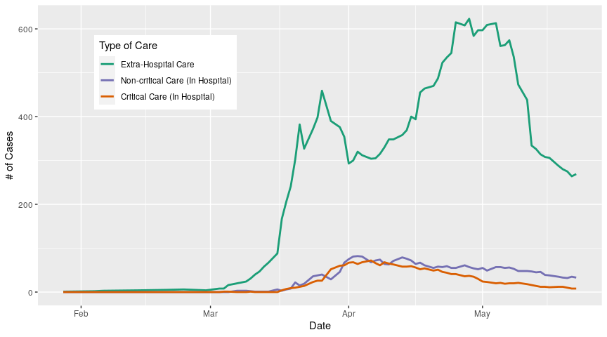
To look at how people are receiving care (in hospital vs. extra-hospital, and critical care vs. non-critical care in hospitals), we need to subtract hospitalized numbers from active numbers:
# I'm also going to use nicer names for the plot legend

treats_drs_long <-
  daily_reports %>%
  select(hosp, IC, self_isolation, date) %>% # select treatment categories
  left_join(cum_drs %>%
              select(date, actives)) %>% # join with current active data
  filter(!is.na(IC)) %>%
  mutate(NC = hosp-IC,
         self_isolation = actives-hosp) %>% # calculate extra-hospitals by subtractive hospitalized patients from active cases
  select(-actives, -hosp) %>% # remove actives because we don't need that data anymore
  gather(key = state, value = cases, -date) %>% # convert to long form
  mutate(state = factor(state, levels = c("self_isolation", "NC", "IC"), ordered = TRUE))

# assign colours manually

care_colours <- RColorBrewer::brewer.pal(3,"Dark2")
names(care_colours) <- c("self_isolation", "IC", "NC")
care_names <- c("Extra-Hospital Care", "Non-critical Care (In Hospital)","Critical Care (In Hospital)")

# plot

ggplot(data = treats_drs_long, aes(x = date, y = cases))+
  geom_line(aes(colour = state), size = 1)+
  labs(colour = "Type of Care")+
  scale_colour_manual(values = care_colours, labels = care_names)+ # assign colours
  theme(legend.position = c(0.1,0.9),
        legend.justification = c(0,1)) +
  xlab("Date")+
  ylab("# of Cases")
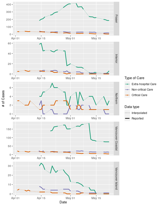
To look at the individual health regions, we need the summary data; the daily reports do provide us the cumulative number of cases at the regional level but they don’t tell us about recoveries or hospitalizations. Unfortunately the summary reports only go back to March 23, and are released less frequently so there are gaps, which for clarity I prefer to indicate on the graphs.
The row labels in the summary report tables are long strings, which can be painful and error-prone to type out when manipulating the data. It’s easier to use abbreviated labels for data catgories, factor levels, treatments, etc., and then have the nice labels standing by for figures. I do that here, by making a csv table with my abbreviated labels and nice labels that I then read in.
# regional data from the summary reports
reg_details <- read_csv("reg_details.csv", trim_ws = TRUE, na = c("","NA"))

# table of nice and abbreviated labels
cat_labs <- read_csv("cat_labs.csv", trim_ws = TRUE, na = c("","NA"))

# join labels to data
reg_details <-
reg_details %>%
  left_join(cat_labs)

# create abbreviations for health regions
map_regions <-
  tibble(reg2 = c("FH", "INH", "NH", "VCH", "VIH"),
         HA_Name = c("Fraser", "Interior", "Northern", "Vancouver Coastal",
                     "Vancouver Island"))

# assign colours manually
reg_colours <- rev(RColorBrewer::brewer.pal(5,"Dark2"))
names(reg_colours) <- c("FH","INH","NH","VCH","VIH")
reg_labs <- c("Fraser", "Interior", "Northern", "Vancouver Coastal", "Vancouver Island")
The data from the summary reports is organized with regions as columns and various case information as rows. We want to calculate the number of active cases in each region for each day that we have data, then use that number to calculate the number of extra-hospital cases. To get to that, we need to filter the data, and then rearrange the table to a format that facilitates our calculations. Once we have the numbers we need, we convert the data back to long form, which is best for plotting.
care <-
reg_details %>%
  filter(cat == "cume_cases" | # filter just the data we want
           cat == "cume_died" |
           cat == "cume_recov" |
           cat == "hosp" |
           cat == "crit_care") %>%
  select(-total, -n, -category, -range, -comments) %>% # select just the regions and date
  gather(key = region, value = n, -date, -cat) %>% # convert to long form
  left_join(map_regions,
            by = c("region" = "HA_Name")) %>% # add region abbreviations
  spread(key = cat, value = n) %>% # convert to wide form with case categories as columns
  mutate(actives = cume_cases - cume_died - cume_recov, # calculate actives
         noncrit_care = hosp - crit_care, # calculate non critical care hospitalized cases
         home_care = actives - hosp) %>% # calculate extra_hospital cases (abbreviated to home_care)
  select(date, region, reg2, home_care, noncrit_care, crit_care) %>% # select just the data we want
  gather(key = care_cat, value = n, -date, -region, -reg2) # convert to long form
We can now go about filling in the gaps in our data.
# make some nice labels for care categories
care_names_list <- c("crit_care" = "Critical Care",
       "home_care" = "Extra-hospital Care",
       "noncrit_care" = "Non-critical Care")

# convert care category to an ordered factor so that when we plot the data as a set of panels, extra-hospital care appears on top.
care <-
  care %>%
  mutate(care_cat = factor(care_cat, levels = c("home_care", "noncrit_care", "crit_care"), ordered = TRUE))

# to fill in the gaps in our data, we need the most recent and earliest dates of the data

most_recent <-
  care %>%
  select(date) %>%
  pull() %>%
  max(.) %>%
  as_date()

earliest <-
  care %>%
  filter(!is.na(n)) %>%
  select(date) %>%
  pull() %>%
  min(.) %>%
  as_date()

# store the difference between the earliest and latest dates

fill_dates_length2 <- 1 + interval(earliest,most_recent) %/% ddays(1)

# use the stored difference in dates to create the "full" combination of dates, regions, and care categories
care_full <-
  tibble(date = rep(seq(earliest, most_recent, by = "day"), each = 15),
         reg2 = rep(c("FH","INH","NH","VCH","VIH"), times = fill_dates_length2, each = 3),
         care_cat = rep(c("home_care", "noncrit_care", "crit_care"), times = 5*fill_dates_length2, each = 1)) %>%
  left_join(care %>% # then join the real data
              select(-region),
            by = c("date" = "date",
                   "reg2" = "reg2",
                   "care_cat" = "care_cat"))

# now to interpolate the missing data
care_gaps <- tibble() # create an empty tibble to store the data

for(i in 1:NROW(map_regions)){ # for each region
  for(k in 1:length(care_names_list)){ # for each care category

    # extract the earliest date for the filtered data
    min_date_gap <-
    care_full %>%
      filter(reg2 == map_regions$reg2[i] & care_cat == names(care_names_list)[k] & !is.na(n)) %>%
      select(date) %>%
      pull(.) %>%
      min(.) %>%
      as_date()

    # identify the dates that are missing data
gaps2 <-
  care_full %>%
  filter(reg2 == map_regions$reg2[i] & care_cat == names(care_names_list)[k] & date >= min_date_gap) %>%
  mutate(rownum = 1:NROW(.)) %>%
  filter(is.na(n)) %>%
  pull(rownum)

gap_brack2 <- vector() # create an empty vector to store the gap positions

# for each identified row that is missing data, store the row number before, row number of missing data, and row number after
for(j in 1:length(gaps2)){
  gap_brack2 <- c(gap_brack2, gaps2[j]-1, gaps2[j], gaps2[j]+1)
}

gap_brack2 <- unique(gap_brack2) # get rid of duplicates (instances where gaps are longer than one day)

# filter the full data set for just the rows missing data and the rows that bracket them, then interpolate
care_gapstmp <-
  care_full %>%
  filter(reg2 == map_regions$reg2[i] & care_cat == names(care_names_list)[k] & date >= min_date_gap) %>%
  mutate(rownum = 1:NROW(.)) %>%
  filter(rownum %in% gap_brack2) %>% # filter for gaps
  mutate(n = na.approx(n)) %>% # interpolate
  select(-rownum) %>%
  left_join(map_regions, by = c("reg2" = "reg2")) %>% # add region names
  rename(region = HA_Name)

# store interpolated data
care_gaps <-
  bind_rows(care_gaps, care_gapstmp)

  }
}

# add region names to full data set
care_full <-
care_full %>%
  left_join(map_regions) %>%
  rename(region = HA_Name) %>%
  mutate(care_cat = factor(care_cat, levels = c("home_care", "noncrit_care", "crit_care"), ordered = TRUE))

# in order for our gap data to plot correctly, we need the dates for which we do have data set to NA and included in the interpolated data tibble
# we do this by taking our full data set, removing the data, and left joining the interpolated data to it
care_gaps <-
care_full %>%
  select(-n) %>%
  left_join(care_gaps) %>%
  mutate(care_cat = factor(care_cat, levels = c("home_care", "noncrit_care", "crit_care"), ordered = TRUE))

# bind interpolated and observed data into one long tibble
care_all <-
bind_rows(care_gaps %>%
            add_column(type = "inter"),
          care_full %>%
            add_column(type = "repo"))

# lastly, there are a couple observed data points that are surrounded by gaps
# these data wont appear on the plot because they are isolated points, there are no lines to draw
# we can plot them as points

singletons <- tibble()
for(j in 1:NROW(reg_labs)){
  for(k in 1:length(care_names)){

    sing_tmp <-
    care_all %>%
              filter(reg2 == map_regions$reg2[j] & care_cat == names(care_names_list)[k] & type == "repo" & is.na(n)) %>%
              mutate(date2 = c(NA,diff(date) == 2)) %>%
              filter(date2 == TRUE) %>%
              select(date, reg2, care_cat, type) %>%
              mutate(date = date - 1) %>%
              left_join(care_all)

    singletons <- bind_rows(singletons, sing_tmp)

  }
}

# plot
ggplot(data = care_all, aes(x = date, y = n))+
  geom_line(aes(colour = reg2, linetype = type, size = type))+
  geom_point(data = singletons, aes(x = date, y = n, colour = reg2), shape = 15, size = 1)+
  facet_wrap(.~care_cat, ncol = 1, scales = "free", strip.position = "right", labeller = labeller(care_cat = care_names_list))+
  scale_linetype_manual(name = "Data type", values = c("dotted", "solid"), labels = c("Interpolated", "Reported"))+
  scale_size_manual(name = "Data type", values = c(0.5, 1), labels = c("Interpolated", "Reported"))+
  scale_colour_manual(values = reg_colours, labels = reg_labs)+
  labs(colour = "Health Region")+
  xlab("Date")+
  ylab("# of Cases")

We can use the same data to plot case categories by region:
# the summary reports-based tibbles use slightly different category names
# need to make a new colour list

care_colours2 <- care_colours

names(care_colours2) <- c("home_care", "crit_care", "noncrit_care")
reg_labs2 <- c("FH", "INH", "NH", "VCH", "VIH")
names(reg_labs) <- reg_labs2

ggplot(data = care_all, aes(x = date, y = n))+
  geom_line(aes(colour = care_cat, linetype = type, size = type))+
  geom_point(data = singletons, aes(x = date, y = n, colour = care_cat), shape = 15, size = 1 )+
  facet_wrap(.~reg2, ncol = 1, scales = "free", strip.position = "right",
             labeller = labeller(reg2 = reg_labs)) +
  scale_linetype_manual(name = "Data type", values = c("dotted", "solid"), labels = c("Interpolated", "Reported"))+
  scale_size_manual(name = "Data type", values = c(0.5, 1), labels = c("Interpolated", "Reported"))+
  scale_colour_manual(values = care_colours2, labels = care_names_list)+
  labs(colour = "Type of Care")+
  xlab("Date") +
  ylab("# of Cases")
To standardize data from each region by population, we can use the population data from BCStats (estimates are from 2019, data licensed under the Open Government Licence - British Columbia).
reg_pops <- read_csv("reg_pops.csv", trim_ws = TRUE, na = c("","NA"))

# keep just totals

reg_pops <-
reg_pops %>%
  filter(cat == "total") %>%
  gather(key = reg2, value = tot, -cat) %>%
  select(-cat)

# left join populations onto care data, calculate cases per 100,000

care_all2 <-
care_all %>%
  left_join(reg_pops) %>%
  mutate(nprop = 100000*n/tot)

singletons2 <-
singletons %>%
  left_join(reg_pops) %>%
  mutate(nprop = 100000*n/tot)

# plot

ggplot(data = care_all2, aes(x = date, y = nprop))+
  geom_line(aes(colour = reg2, linetype = type, size = type))+
  geom_point(data = singletons2, aes(x = date, y = nprop, colour = reg2), shape = 15, size = 1)+
  facet_wrap(.~care_cat, ncol = 1, scale = "free", strip.position = "right", labeller = labeller(care_cat = care_names_list))+
  scale_linetype_manual(name = "Data type", values = c("dotted", "solid"), labels = c("Interpolated", "Reported"))+
  scale_size_manual(name = "Data type", values = c(0.5, 1), labels = c("Interpolated", "Reported"))+
  scale_colour_manual(values = reg_colours, labels = reg_labs)+
  labs(colour = "Health Region")+
  xlab("Date")+
  ylab("# of Cases per 100,000") #+
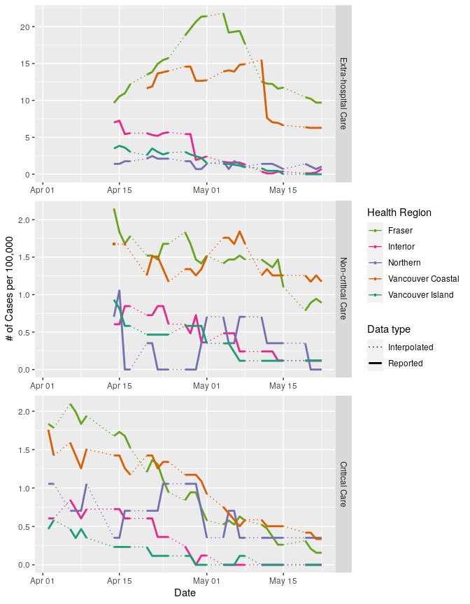
Et voila!
All analyses performed in R V3.6.3